All published articles of this journal are available on ScienceDirect.

Prognostic Genomic Predictive Biomarkers for Early-Stage Lung Cancer Patients
Abstract
Aims:
Our goal is to find predictive genomic biomarkers in order to identify subgroups of early-stage lung cancer patients that are most likely to benefit from adjuvant chemotherapy with surgery (ACT).
Background:
Receiving ACT appears to have a better prognosis for more severe early-stage non-small cell lung cancer patients than surgical resection only. However, not all patients benefit from chemotherapy.
Objective:
Preliminary studies suggest that the application of ACT is associated with a better prognosis for more severe NSCLC patients compared to those who only underwent surgical resection. Given the immense personal and financial costs associated with ACT, finding the patients who are most likely to benefit from ACT is paramount. Thus, the purpose of this research is to utilize gene expression and clinical data from lung cancer patients to find treatment-associated genomic biomarkers.
Methods:
To investigate the treatment effect, a modified-covariate regularized Cox regression model with lasso penalty is implemented using National Cancer Institute gene expression data to find genomic biomarkers.
Results:
This research utilized an independent validation dataset involving 318 lung cancer patients to validate the models. In the validation set with 318 patients, the modified covariate Cox model with lasso penalty were able to show patients who followed their predicted recommendation (either ACT for low-risk group or OBS for the high-risk group, n = 171) have higher survival benefits than 147 patients who did not follow the recommendations (p < .0001).
Conclusion:
Based on validation data, patients who follow our predicted recommendation by genomic biomarkers selected from the proposed model will likely benefit from ACT.
1. INTRODUCTION
The task of identifying subgroups that are more likely to benefit from a particular treatment falls into the realm of causal inference and precision medicine. There is an increase in medical interest focusing on providing personalized care for patients. This requires investigating how unique patient characteristics, which may include both clinical and genetic, impact treatment efficacy. A better understanding of the interaction between treatment and patient-specific predictive factors will enable medical practitioners to build upon the availability of individually tailored and optimal therapies. Ultimately, the goal is to build individual-specific decision support tools that enable a data-driven understanding of the treatment options and improve patient outcomes.
Non-Small Cell Lung Cancer (NSCLC) is the leading cause of cancer-related deaths worldwide. For early-stage lung cancer patients, surgical resection only is the most common treatment. For more severe patients, several randomized control studies involving patients with resected stages IB to IIIA, NSCLC have indicated cisplatin-based adjuvant chemotherapy (ACT) significantly benefitting 5-year survival rates, with improvements ranging from 4% to 15% [1]. Despite the limited improvement in survival, ACT remains a demanding procedure, and the toxicity associated with the treatment facilitates careful consideration on an individual level whether the potential benefits outweigh the risk and cost. Toxic side effects occurred from chemotherapy treatment in a large portion of ACT-treated patients in a study [2, 3]. This included neutropenia (88%), fatigue (81% of patients), nausea (80%), and anorexia (55%). Neutropenia was the most common severe side effect of the ACT treatment; 73% of patients had grade 3 or grade 4 neutropenia. These typical side effects of chemotherapy again emphasize the need for careful consideration to ensure patients who will actually benefit from chemotherapy and should receive ACT.
Recent technological advances in the realm of genetics allow for high throughput gene expression profiling at the molecular level in a relatively cost-efficient manner. Thus, the increasing availability of microarray data has given rise to the field of bioinformatics and countless opportunities to mine through such data with applications, especially in the fields of disease classification and drug discovery. At present, the use of prognostic gene expression data in formal clinical practice is still an ongoing process.
The goal of this analysis is to use gene expression profiling to identify genomic biomarkers for stage-independent groups of NSCLC patients, who are more likely to benefit more from ACT than surgical resection only. This could help lead to more accurate and optimal treatment decisions, thereby improving the efficacy of ACT and avoiding unnecessary toxicities and costs.
Many previous studies have sought to identify prognostic gene signatures in NSCLC patients. A previous gene expression study by Raponi et al. was able to discover prognostic gene signatures that were correlated to NSCLC patient survival [4]. In particular, Zhu et al. identified a 15-gene prognostic signature using data from patients who underwent surgical resection only (OBS patients) to classify patients into a low-risk and high-risk category with respect to overall survival [3]. We note that their predictive results utilized the same OBS patients that they trained their model with, thus possibly introducing bias into their results. We used a separate validation set to minimize over-fitting and provide an unbiased evaluation of our model.
Decision tree-based ensemble methods have been popular within literature due to their relatively simple and interpretable nature. Foster et al. suggested utilizing a two-stage “virtual twins” model for subgroup identification for randomized controlled trials [5]. The model first utilizes random forest models to estimate the treatment effect for each patient. Then, it applies the Classification and Regression Tree (CART) algorithm [6] to determine a small number of predictors that were associated with the treatment effect. This model was shown to perform well on clinical trial data and simulated data, verified through different validation methods. Recently, Moon et al. developed their methods similar to a two-stage virtual twin’s model for subgroup analysis of NSCLC patients [7].
Previous work by Moon et al. also tackled the problem of predicting the treatment recommendation for NSCLC patients [7, 8]. Their methods implemented two prediction models based on two treatment groups (ACT and OBS) using the training data. They employed feature selection with the lasso penalty and later with the net elastic penalty. Then, they both utilized Accelerated Failure Time (AFT) models separately on each group to estimate whether the patients would survive longer under ACT treatment. They specifically used a two-stage random forest method for the classification but did not validate their results on an independent test set. A potential drawback from their approach might be that they implemented two models by splitting the patients into two groups with one that received chemotherapy treatment and one without and trained two separate sets of patients. By decreasing the training sizes for the two patient groups, it might introduce the risk of overfitting the models and increase the chance of selecting false-positive features. Another potential drawback might be the implementation of the two-stage random forests method. Their overall model could only predict if a patient should undergo chemotherapy when both random forest models classified the patient with the same prediction. Thus, patients with differing predictions from the two random forests were inconclusive for an overall prediction.
The previously mentioned studies motivate further exploration into utilizing gene expression data in a clinical setting. In this paper, we propose a modified covariate approach that combines the problem into a single framework. The proposed models introduce explicit treatment interaction factors for identifying genes that are closely related to the treatment effect. Unlike the studies mentioned previously, a separate validation set is used to evaluate model performance.
2. DATA DESCRIPTION
The JBR.10 data set utilized by Zhu et al. [3] comes originally from a large-scale randomized study by Winton et al. [2], comparing the survival of early-stage NSCLC patients that underwent adjuvant vinorelbine/cisplatin versus observation alone. The goal of the study was to determine whether patients with completely resected non-small-cell lung cancer receive survival benefit from adjuvant vinorelbine plus cisplatin treatment. In the original study that began in July 1994, a total of 482 patients randomly received a treatment of either surgery alone with no chemotherapy (n = 242) or a regimen of ACT treatment following surgery (n = 240).
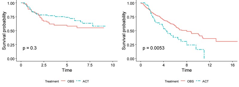
As Zhu et al. utilized the data, 133 randomly selected frozen JBR.10 tumor samples were used as a training dataset in this paper [3]. Among the 133 patients with gene expression profiles using the Affymetrix U133A oligonucleotide microarrays [9], 71 patients received chemotherapy, and 62 received surgery only. The median age was 62 years old, and 68% of the patients were men. 55% of the patients were stage IB, and 45% were stage II. 53% of the patients had adenocarcinomas, 39% had squamous cell carcinomas, and 8% had another type of cancer. In the training set, patients in the chemotherapy group exhibited slightly higher survival than those in the observation group after around 2 years (Fig. 1). For the training set, the 5-year survival rate for the chemotherapy group was 73.7%, while it was 57.9% for the observation group. The hazard ratio between ACT and OBS was 0.74 (p = .3), meaning that ACT treatment has a 26% lower risk of death than OBS treatment alone. This JBR.10 dataset was downloaded from the NCBI website with the accession number GSE14814 and was used as the training set (https://www.ncbi.nlm.nih.gov/geo/query/acc.cgi?acc=GSE14814).
For the validation set, data was used from the Director's Challenge Consortium for the Molecular Classification of Lung Adenocarcinoma (DCC)— a large retrospective microarray study of lung adenocarcinoma survival rates using a gene expression data from Shedden et al. [10]. Lung samples from a total of 442 patients with adenocarcinoma were collected from across four institutions. Since 43 of the DCC samples were found in the JBR.10 dataset, they were excluded to ensure independence between the training and validation data in this paper. To ensure further concordance between both the training and validation sets, patients with Stage III lung cancer were removed from the DCC samples since the JBR.10 samples only consisted of Stage I and Stage II patients. After removing samples with missing values on treatment and time to follow up/death covariates, 318 samples remained as a validation set. This validation set was downloaded from the NCBI website with the accession number GSE68465 (https://www.ncbi.nlm .nih.gov/geo/query/acc.cgi?acc=GSE68465).
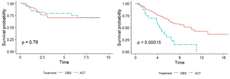
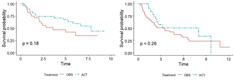
Demographics for the patients used in both training and validation sets are summarized side-by-side in Table 1. Overall, for patients in the validation set, the OBS patients exhibited higher survival than the chemotherapy patients, possibly due to the toxicity of ACT (p = 0.005), (Fig. 1). When split by stage, Stage I patients in the validation set showed much higher survival if they underwent surgery only (p < 0.001), (Fig. 2). It may be due to the high proportion of stage I patients. On the other hand, Stage II patients in the validation set showed only marginally higher survival if they underwent chemotherapy (p = 0.26), (Fig. 3). Thus, in this paper, we focus on individualized treatment by building a modified covariate Cox regression model with lasso penalty to identify genomic biomarkers in order to maximize patient survival.
3. METHODS
3.1. Data Preprocessing
The Affymetrix microarray is a device designed to simultaneously measure the expression levels of thousands of genes in a particular tissue or cell type of interest. The microarrays are microscopic slides that are printed with thousands of tiny spots in defined positions, with each spot containing known DNA sequences that correspond to particular genes. The DNA molecules attached to each slide act as probes to detect gene expression from incoming samples, which is also known as the transcriptome or the set of messenger RNA (mRNA) transcripts expressed by a group of genes. Specifically, for the U133A GeneChip used in the analysis, there are over 14,500 detectable genes. For each of the detectable genes in the array, there is a corresponding probe set containing 11 distinct 25-base pairs. The 11 distinct pairs include a perfect match (PM) probe and a complementary mismatch (MM) probe. The PM probe is designed to match a particular sequence of interest perfectly, while the MM probe is designed to measure the level of mis-hybridization. Together, they help provide a more accurate measurement of gene expression.
Before any initial analysis may begin, the raw microarray data must first be preprocessed as a set of intensities by usually following three steps, background correction, normalization, and summarization. Preprocessing procedures combine multiple probe signals into a single value. There are inherent physical differences between each microarray chip as well as differences in the handling of the chip and internal dye intensity effects that introduce extraneous noise to the data. Thus, a problem arises when true biological variation in the microarray chips becomes entangled with an unwanted systematic variation. Background correcting procedures adjust the values for the ambient background intensities in each probe. Since the probes are usually randomly scattered within the microarray, there should not be any particular spatial pattern in the intensities. It removes local artifacts and noise so that the measurements are not so affected by neighboring measurements. For robust multichip average (RMA) method, background correction involves modeling the observed Perfect Match (PM) signal of each probe as a sum of an exponentially distributed true signal (S) term and a normally distributed noise term (e):
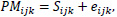 |
where the index i represents the particular sample or microarray, index j represents the probe pair (within each probe set corresponding to a particular gene), and index k represents the particular gene within the microarray. From this, the expected value of the true signal intensity given the observed PM signal, E(Sijk|PMijk), is estimated as the background-corrected intensity.
Normalization is required to correct and compensate for the unwanted variation and scale the distribution of the gene expression so that actual biological differences in the gene expression may be more appropriately detected. Quantile normalization is a standardizing technique to make similar distributions. As an example, consider three microarrays with 4 probes. Array 1 has values {3, 5, 6, 7} for 4 probes, array 2 has {9, 9, 3, 6} and array 3 has {6, 3, 7, 4}. The first step is to rank the values within each array. Array 1, 2, and 3 have ranks {1, 2, 3, 4}, {3.5, 3.5, 1, 2}, and {3, 1, 4, 2}, respectively. The second step is to obtain averages of each rank across arrays. Rank 1 average is (3+3+3)⁄ 3=3; rank 2 average is (5+6+4) ⁄ 3 =5; rank 3 average is (6+9+6) 3 = 7; rank 4 average is (7+9+7) ⁄3=7.67. The last step is to replace the average rank values with the rank position in each array. Thus, normalized array 1 has values {3, 5, 7, 7.67}. For normalized array 2, we use the average value of rank 3 average and rank 4 average due to a tie. Thus, normalized array 2 has {7.335, 7.335, 3, 5} values. Normalized array 3 has {7, 3, 7.67, 5} values.
Finally, the summarization step combines probe intensities across the probe set into a single value that may be considered the gene expression level. The summarization step involves using background-corrected and normalized intensities and their logged values. These log-transformed intensities denoted as Yijk, is then modeled as the following linear additive model:
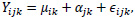 |
where µik represents the log scale expression level for microarray i for gene k, á jk is the probe affinity effect for probe pair j and gene k, and ϵijk is the independent identically distributed error term. Given the noisy nature of gene expression data, the median polish method developed by Tukey [11] is utilized to estimate the parameters on the right-hand side in the additive model. The median polish method involves iteratively extracting row and column medians to estimate the row and column effects that correspond to the microarray and probe pair effects, respectively. The estimate of µik gives the final RMA expression measure for microarray i and gene k.
By continuing with the previous example, the final RMA expression measures for the probe set via the median polish method is calculated as follows: for the normalized array 1, {3, 5, 7, 7.67}, the median is 6 across the probe set. For the normalized array 2, {7.335, 7.335, 3, 5}, the median is 6.1675. For the normalized array 3, {7, 3, 7.67, 5}, the median is 6. After removing the row medians obtained across the probe set, the array 1 has values {-3, -1, 1, 1.67}, the array 2 has {1.1675, 1.1675, -3.1675, -1.1675} and the array 3 has {1, -3, 1.67, -1}. Now we obtain column medians across arrays per each probe. Medians for probes 1, 2, 3, and 4 are 1, -1, 1, and -1, respectively. After removing the column medians, the residual values for arrays 1, 2 and 3 are {-4, 0, 0, 2.67}, {.1675, 2.1675, -4.1675, -.1675}, and {0, -2, .67, 0}. The median polish algorithm stops because all row medians and column medians are zero. To obtain the RMA expression measure for each of the three arrays, the residual values are subtracted from the original values. Thus, the resulting expression values for arrays 1, 2, and 3 are {7, 5, 7, 5}, {7.1675, 5.1675, 7.1675, 5.1675}, and {7, 5, 7, 5}. By taking the mean across each probe set, the RMA expression measures for the three arrays are found to be 6, 6.1675, and 6.
The raw CEL files from both datasets were preprocessed and normalized altogether via the RMA algorithm to ensure consistency between the datasets using the “Affy” package in R [12]. The dataset contains over 23,000 probe sets which warranted an initial variable screening. Nonspecific gene filtering is a popular technique to help alleviate the high dimensional nature of genetic data by keeping only the probe sets that show high variability and remove low variability probe sets that are likely non-informative. This should help with potential overfitting with the removal of false positives and redundant covariates for more efficient analysis. Affymetrix microarrays contain control probe sets (denoted by the “AFFX” prefix) that do not correspond to any particular genes and are used to help normalize gene intensities. These control probe sets are thus removed before performing gene filtering. Nonspecific gene filtering is then applied in the analysis, keeping only the 10,000 probe set features with the highest variance in the training dataset. Thus, the features used to train the model are the remaining 10,000 probe sets in addition to the demographic and clinical covariates of age, sex, and stage.
3.2. Statistical Methods
Survival analysis models the expected duration of time until an event occurs, whether it is the death of a biological entity, recurrence of a disease, or failure of a mechanical system. Survival modeling involves examining the relationship between survival time data, which is commonly subject to censoring, and one or more covariates.
The Cox proportional hazards model is a popular choice to model covariates in relation to a survival time due to its relative simplicity and convenience in handling censored observations [13]. Given the survival data (ti, δi, Z i), i = 1, … n, where ti is the observed survival or censored time, δi is the censoring indicator for the survival time, and Zi = (Zi1, Z i2, …, Zip)T is a p -dimensional covariate vector for the ith individual, the Cox model is
 |
where λ(t|Z) is the hazard rate at time t given the covariates Z, λ0(t) is the baseline hazard rate, and β is a p-dimensional parameter vector associated with each of covariates. Cox [13] proposed the partial likelihood to estimate the parameters β through the following formula:
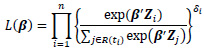 |
The estimated parameters for the cox model are given by minimizing the partial likelihood, which is given as:
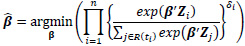 |
where R(ti) = {j: tj ≥ ti} denotes the risk set at time ti. Only uncensored event times contribute their own factor to the partial likelihood. However, both censored and uncensored observations appear in the denominator, where the sum over the risk set includes all individuals who are still at risk immediately prior to ti. The proportional hazards condition states that covariates are multiplicatively related to the hazard; the model itself does not directly estimate survival times but rather estimates how the covariates affect the hazard rates. The logarithm of the partial likelihood is minimized due to the ease of calculation. This is given as:
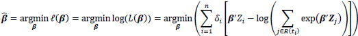 |
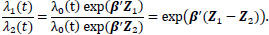
The survival of two individuals can be compared with hazard ratios; given two individuals with covariates Z1 and Z2, the hazard ratio between the two individuals is given by
 |
Because the number of covariates greatly outnumbers the number of observations in high dimensional microarray data, overfitting and high variance may be significant problems. Thus, additional consideration must be taken to select the most relevant covariates. Tibshirani proposed extending the lasso penalty in the least-squares regression models into the context of Cox models by minimizing the partial likelihood with the lasso [14]. The lasso estimates for the Cox model are
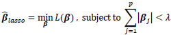 |
where γ is a specified penalty parameter and p is the number of covariates. The nature of the lasso constraint causes it to shrink irrelevant coefficients and produces coefficients that are exactly zero. As a result, it simultaneously reduces the estimation variance while providing a final interpretable model with a feasible set of variables. If too large of a penalty parameter λ is chosen, the estimated parameters
 maybe significantly biased; if too small, the model may not be sufficiently sparse. In some circumstances, one may not want to eliminate certain covariates with the lasso penalty from the model during training if the covariates hold some underlying importance or special weight in regard to the response. This may be done by modifying the minimization problem above:
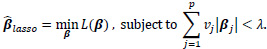 |
By adding an individual penalty term vj for each coefficient j, chosen coefficients may be left out of the regularization process even if the penalty term vj is zero. Thus, this prevents the specified covariates from being removed by the lasso penalty in the final model.
We employ the modified covariate method by Tian et al. [15]. A set of q covariates (both clinical and genetic data) Z, and a binary treatment variable T, which takes on values of -1 or +1 corresponding to observation or treatment, respectively, are given. Let function W be p dimensional functions of covariate Z including an intercept. To identify the subgroup of patients who may or may not benefit from the treatment, we consider a treatment interaction term. Thus, the modified covariate method begins with
 |
where W*i = W(Z)∙ T2. For simplicity in this analysis, W(Zi) is chosen as the identity function, W(Zi) = Zi. For survival data, the following Cox regression model can be used:
 |
Under the modified covariate approach, the linear combination γTZ can be thought of as a treatment score and thus used to stratify patients according to how they would respond to a treatment. For example, if given T = + 1 as ACT treatment, higher treatment scores γ T Z correspond to a higher hazard, and thus ACT treatment is not recommended. On the other hand, lower treatment scores correspond to a relatively lower hazard, and thus ACT may be recommended. In the randomized trials, we assume P(T=1) = P (T= - 1) =
 meaning that the treatments are randomly assigned to each patient.
The features are transformed to the modified covariate approach, where each feature is multiplied by the corresponding treatment (either T/2 = + 0.5 or T/2 = - 0.5). The modified covariate Cox model is then trained using the preprocessed JBR.10 training set. We note that the coefficients associated with the modified covariate measure the interaction strength between treatment and subgroup of patients who may or may not benefit from the treatment. To further reduce the dimensionality and alleviate high potential variance, the model is trained using the lasso regularization penalties to select prominent predictive genomic markers. Given the potential importance of the clinical covariates, the model trained with the lasso is modified to keep the three clinical covariates in the model. We implement this approach using the glmnet package in R, which uses the coordinate descent algorithm to approximate the penalized coefficient estimates. Then, the results from both regularization methods are compared. Due to the nature of the relatively small training set, a Leave-One-Out Cross-Validation (LOOCV) scheme was used to tune the lasso penalty parameter. The LOOCV is a popular variant of k-fold cross-validation involving the splitting of samples randomly into k groups or folds. The standard approach for the LOOCV is made by setting aside one observation as the testing sample and fitting the model on the remaining n - 1 observations in the training sample. Then, the model evaluation is made on the left-out testing sample. This process is repeated for each of the observation, where each fold is served as the testing set once. Ultimately, the hyperparameters that maximize the average of the cross-validation metrics are chosen. This helps determine the optimal model hyperparameters so that the model is not overfitted on the training data.
In the Cox regression framework where there is censoring, maximizing the partial likelihood may lead to a problem when the testing sample used for cross-validation is too small. If the number of testing samples is too small, there may not be enough samples to build up an appropriate risk set R(ti) present in the partial likelihood. This could potentially lead to undefined or unstable partial likelihoods. Verweij and Van Houwelingen [16] proposed a method to calculate a shrinkage factor by measuring CV score, mentioned as below:
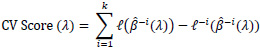 |
where
 refers to the partial likelihood calculated on the entire dataset,
 refers to the partial likelihood on the dataset which excludes the i-th observation (out of n observations), and
-i (λ) refers to the estimated parameters fitted using the training set, which excludes the left-out observation and the using candidate λ parameter. This avoids calculating the partial log likelihood directly on the held-out testing set and ensures a sufficient number of samples to be defined for the partial likelihood.
refers to the partial likelihood on the dataset which excludes the i-th observation (out of n observations), and
-i (λ) refers to the estimated parameters fitted using the training set, which excludes the left-out observation and the using candidate λ parameter. This avoids calculating the partial log likelihood directly on the held-out testing set and ensures a sufficient number of samples to be defined for the partial likelihood.
After training, the estimated parameters
maybe used to find the risk scores (risk with respect to ACT treatment) for the training set given by
'Z. A threshold must then be determined to stratify the patients into a low-risk and high-risk group. Patients who have a risk score higher than the threshold are classified as high-risk patients and thus are not recommended chemotherapy treatment; conversely, patients whose risk scores are lower than the threshold are classified as low-risk patients and thus are recommended chemotherapy treatment.
One possible and natural choice is to set the decision threshold at zero. By using the modified covariate approach, the hazard ratio of the two treatments on an individual is given by:
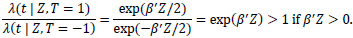 |
If the patient risk score β'Zi> 0, then the hazard rate is greater if the patient undergoes T = + 1 (which corresponds to ACT treatment) than if the patient does not. Conversely, if the risk score β' Zi< 0, then the hazard rate for the patient is lower had they undergone ACT treatment compared to without ACT treatment. Setting the threshold to zero is a sensible choice under the assumption that the modified covariate method is indeed the actual model of interaction between treatment and the other covariates. Even though setting the decision threshold at zero may only capture the relative direction and not the size of the effect, we considered both zero risk score and the median of the risk scores as thresholds in order to make predicted treatment recommendations by classifying patients into a high or low-risk group. To evaluate the classifier, survival curves are used based on treatment types and classified risk groups. For example, for the patients classified in the high-risk group, those who underwent ACT should be expected to survive just as short or shorter than those who did not. Conversely, in the low-risk group, patients that underwent ACT are expected to survive longer or just as long as those who did not.
Additionally, patients may further be separated into the following two groups: one where the actual treatment they underwent corresponded to the treatment recommended according to their predicted risk group and the other where the two do not correspond. For a particular patient i, if TXi represents the actual treatment that patient i received and Ri is the recommended treatment based on the previous risk scores, then the variable Fi indicating whether the patient i followed the recommended treatment is given by
 |
A successful classifier, in principle, should split the patients such that those who follow the recommendation exhibit higher survival than those who do not. Finally, the modified covariate model trained using the JBR.10 dataset is validated using the DCC dataset.
4. RESULTS AND DISCUSSION
After tuning the lasso penalty λ with LOOCV, the modified covariate Cox model is built with the chosen lasso penalty on the entire training set. The covariates of age, stage, and gender are explicitly left unregularized and are present in the final model. Table 2 shows the selected genomic markers by the lasso penalty. Those probe sets significantly interact with the treatment.
All genes selected from the lasso show a potential relationship with NSCLC and/or ACT from literature. AKR1C3 has previously been found to be overexpressed specifically in NSCLC and can be used to determine NRF2 (Nuclear factor erythroid 2-related factor 2) status [17]. Determining NRF2 status is vital because activation of the NRF2 pathway has been previously discovered to be correlated with benefit from adjuvant chemotherapy for NSCLC patients [18]. The inhibition of genes in the G-antigen family of lung cancer patients has been found to result in a more sensitive reaction to drugs used in adjuvant chemotherapy like cisplatin and etoposide [19]. Recent studies suggest that the overexpression of the PROM1 gene is associated with a poorer prognosis of NSCLC [20]. In addition, it has been proposed that the CLIC3 gene is a prognostic biomarker for lung cancer [21]. DHRS2 has also been previously found to be correlated with metabolism proteome clusters and overall survival in NSCLC patients [22].
| Probe Set/Covariate | Gene Symbol | Gene Name |
| 209160_at | AKR1C3 | aldo-keto reductase family 1 member C3 |
| 207739_s_at | GAGE2D, GAGE2E, GAGE2A, GAGE13, GAGE2B, GAGE2C, GAGE12D, GAGE4, GAGE12J, GAGE10, GAGE1, GAGE8. | G – antigen family |
| 204304_s_at | PROM1 | prominin-1 |
| 214079_at | DHRS2 | Dehydrogenase/reductase SDR family member 2 |
| 219529_at | CLIC3 | Chloride intracellular channel protein 3 |
We implemented the modified covariates model using the lasso penalty with the JBR.10 dataset as the training set and stratified the patients along the median of the estimated risk scores from the model; 67 of the training set patients were classified as the low-risk group, and the remaining 66 as the high-risk group. For the low-risk patients, ACT treatment was recommended, while for the high-risk patients, ACT was not recommended. The survival analysis was conducted between a group of patients who actually followed the predicted recommendation and a group of patients who did not follow the predicted recommendation. There were 75 patients who actually underwent the predicted treatment, and the remaining 58 patients had discordance between their actual treatment and their predicted treatment. The log-rank test showed significantly higher survival for the patients who followed the predicted treatment than patients who did not follow it (p<0.001;) (Fig. 4), thus indicating that the model performed well on the data that it was trained on.
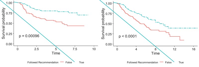
Similarly, 159 patients in the validation set were classified into the high-risk group and the remaining 159 into the low-risk group by the modified covariate model with the lasso penalty using the median risk score. Among them, 161 patients actually followed their predicted treatment recommended by the model, and the remaining 157 patients did not. The model exhibited a significant survival difference between the two groups (p<0.0001), (Fig. 4). This showed stronger evidence in the efficacy of the treatment recommended by the model and the ability of the estimated risk scores to stratify patients into subgroups that are likely and not likely to benefit from chemotherapy.
We also implemented the lasso penalty model with a zero cut-off threshold to classify the patients in the validation set into high-risk and low-risk subgroups for predicting treatment recommendations. The model classified 189 patients as low risk and 129 as high risk. The 151 patients who followed predicted treatment recommendations from the model also showed very similar survival patterns to (Fig. 4) and showed significantly higher survival than 167 patients who did not (p<0.0001).
CONCLUSION
The aim of this paper is to provide an individualized treatment recommendation to early-stage lung cancer patients by finding a potential treatment-related set of genomic biomarkers using the lasso Cox regression model with modified covariates approaches on the survival of lung cancer patients. The JBR.10 data set, consisting of randomly selected 133 frozen tumor samples, was used as the training set. These 133 patients were comprised of 71 who received chemotherapy and 62 who received surgery only, with 55% of them in stage IB and 45% in stage II. For the validation set, the DCC dataset of lung samples from 442 patients was used. Among 442 samples, 43 samples were removed because they were part of the training set, and other samples were removed to maintain consistency of the only Stage I and Stage II patient samples or were removed due to missing treatment and time to follow up/death covariates, ultimately leaving 318 samples for the validation set.
Given the specific nature of collecting gene expression data, a source of potential variation arises from how the gene expression data is obtained. Unwanted nonbiological variation may be caused by different procedures and methods of handling specimen to the laboratory where the data is collected or by the researcher who collects the data. Thus, we use the Robust Multichip Average (RMA) method to normalize the training and validation datasets. We note that the validation set used in this analysis contains only lung adenocarcinomas.
By implementing lasso conditions to help prevent overfitting and reduce model variance given the high-dimensional nature of the genomic data, risk scores were estimated by the regularized Cox regression model at the individual patient level. The scores were stratified patients into low-risk and high-risk groups respective to chemotherapy treatment. Low-risk patients were recommended ACT by the model, while high-risk patients were recommended OBS. To find the optimal penalties in the lasso method, a LOOCV scheme was implemented by using a modified cross-validation score for the survival data. Within the JBR.10 training set, 65 patients who followed the predicted recommendation by the model exhibited significantly higher survival than 68 patients who did not follow the predicted recommendation (
Besides age, stage, and gender as clinical and demographic covariates, a set of potential genomic markers were selected by the proposed model. Those selected probe sets significantly interacted with the treatment showing a potential relationship between NSCLC and chemotherapy. For example, the overexpression of the PROM1 gene appeared to be associated with a poorer prognosis of NSCLC [20]. The CLIC3 gene has been previously identified as a prognostic NSCLC biomarker [21]. Similarly, G-antigen family genes appear to determine sensitivity to drugs like cisplatin and etoposide that are used in adjuvant chemotherapy [19].
This research utilized an independent validation dataset involving 318 lung cancer patients to validate the models. In the validation set with 318 patients, the modified covariate Cox model with lasso penalty were able to show patients who followed their predicted recommendation (either ACT for low-risk group or OBS for the high-risk group; n = 171) have higher survival benefits than 147 patients who did not follow it (p <.0001). The lasso penalty produced a resulting parsimonious model. The results on the validation set suggest that the presented modified covariate regularized Cox regression model with the lasso penalty shows a convincing outcome in determining the benefit from personalized treatment.
The clinical and demographic covariates in this paper were limited to the ones present in the JBR.10 training set, which consisted of lung cancer stage, patient age, and patient sex. Future studies may incorporate more clinical covariates to determine treatment interactions, given that many clinical covariates directly correlate with patient health. Neutropenia is a severe side effect of chemotherapy treatment, and for this, an example of a potential critical covariate would be the White Blood Cell Count (WBC) or Complete Blood Count (CBC) of a patient that should be incorporated.
ETHICS APPROVAL AND CONSENT TO PARTICIPATE
Not applicable.
HUMAN AND ANIMAL RIGHTS
Not applicable.
CONSENT FOR PUBLICATION
Since the datasets were publicly available, it is not applicable.
AVAILABILITY OF DATA AND MATERIALS
The datasets for the current study are available from the NCBI website with the accession number GSE14814 (https://www.ncbi.nlm.nih.gov/geo/query/acc.cgi?acc=GSE14814for the training set and with the accession number GSE68465 (https://www.ncbi.nlm.nih.gov/geo/query/acc.cgi?acc=GSE68465) for the validation set.
FUNDING
This research was partially supported by the Research, Scholarship, and Creative Activity (RSCA) Award from CSULB.
CONFLICT OF INTEREST
The authors declare no conflict of interest, financial or otherwise.
ACKNOWLEDGEMENTS
We thank CSULB for their help in the research.